Are you tired of users (even yourself) mis-typing data in Excel cells, breaking your lookup formulas? Do you want to select from a list of items to reduce typing and copy/paste?
You probably saw Excel worksheets where you click on the “down” arrow and get a list. This quick guide will help you do it and reveal a few tips and tricks to make your life easier.
Getting started with data validation and in-cell dropdowns
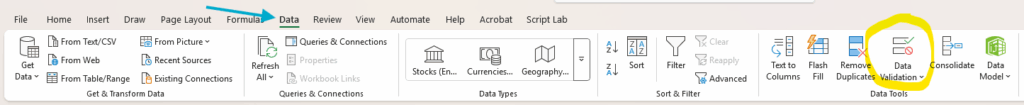
In-cell dropdowns start with “Data Validation”. This limits the data a user can enter in a cell. It is available in the “Data” ribbon, within Microsoft Excel:
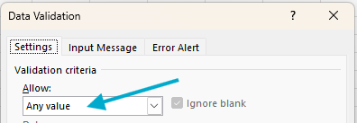
Click on the Data Validation button and you get the “Validation criteria” window, where you choose what to allow. By default, it is “Any value”:
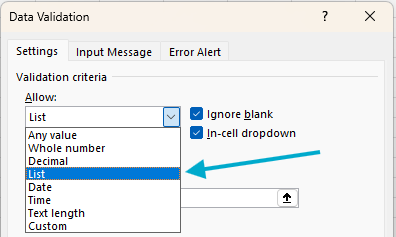
For in-cell dropdown lists, select “List” from the “Allow” options:
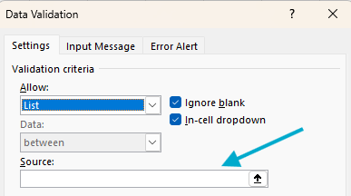
Then, in the “Source” field, enter the list of data to choose from:
Note also the “In-cell dropdown” checkbox: it must be checked to get an in-cell dropdown (this is the default). You have few ways to enter the Source, and I will provide some tips about it. I start with the most scalable approach and I present some shortcuts later.
The best way: use tables and named ranges
The best way to set the source for a data validation list is:
- Create a Table
- Create a Named Range inside the table
- Use the named range as the Source in the Data Validation window
Let’s explain this step by step.
A short introduction to Tables
First, let’s explain an often misunderstood feature in Excel: Tables.
For many users, Tables is only a cosmetic feature. This misunderstanding may be due to the choice of words on the button: “Format as Table”:
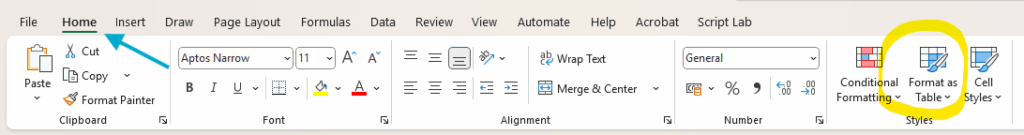
In reality, “Format as Table” does a lot more than pleasing the eye. Internally, Excel handles Tables very differently to Ranges. This improves data validation lists, among other things. If you want to understand tables better, you can read more about them here. For now, let’s see how they affect Data Validation.
Set up a Table for Data Validation
To prepare the table, follow these steps (or check the video below):
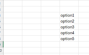
- Enter a title and, underneath, the list of values you wish to use. Skip the first row: start from the second row, or lower.
- Select the cells where you entered the values, including the title.
- Click “Format as Table” in the ribbon. In the popup that comes up, select “My Table has headers”.
- Use the “Table Name” field in the “Table Design” ribbon (it appears when a Table cell is selected) to rename your table to be something meaningful. I apply the “tbl” prefix, shorthand for “table”.
- Then, hover the mouse close to the top boundary of the table’s header, until it becomes a black arrow pointing down. Click, and the cells under the title will be selected. This is easier if the table does not start at the top row, or the black arrow can select the entire worksheet column. If this happens, click somewhere else and try again.
- With the cells under the title selected, click in the Name Box (the cell right above Column A, where you find the address of the selected cell) and type a name. This creates a named range, and this will also be the name of your data validation list. I usually use the same name as the table title, but with a “lst” prefix instead of “tbl”: if the title is “Title”, the table name would be “tblTitle” and the range name “lstTitle”.
Check it out:
Use the Table for data validation
You can now use the Table you just created for data validation. Start where we left off earlier, the Source field in the Data Validation window:
Type the equal sign (=) followed by the name of the range you created (noted as “lstTitle” above) in the “Source” field. Then click ok and the in-cell dropdown is ready to use:
This approach has the following benefits:
- Using a named range makes it much easier to track data validation lists, as you can choose meaningful names. You could accomplish the same by creating a named range outside a table, but using a table brings a second advantage.
- The named range within the table makes it expand automatically if you add values at the bottom. It may not sound as much, yet it makes it expanding your data validation list much easier, when needed later, and helps avoid errors.
Upgrade your lists with Power Dropdown
Using the tips explained above, your in-cell dropdown lists will scale well, helping you create and maintain even complex workbooks without worrying much about errors.
To make your in-cell dropdown lists even more powerful, consider using the Power Dropdown add-in:
- It displays the list in a popup window, making it more user-friendly.
- It extends the list to the entire table column, if your data validation list is inside a table.
- You can display additional text (a “label”), next to the selectable value, to help users choose.
- The values can be deduped taking labels into account.
- You can filter the list by typing. If you added labels, the filter also applies to them.
- A button can take you to the data validation list, very handy if you have many of them.
- With the Premium version, you can also pre-define filters, to shorten the list.
Check it out:
Lazier in-cell dropdowns
The method explained above, using tables and named ranges, is the safest and most scalable way to create in-cell dropdown lists. But I admit it is laborious and it can be tempting to skip some steps. Here, I explain some shortcuts you can take, and their consequences.
Skipping the Table: using a range as the Source
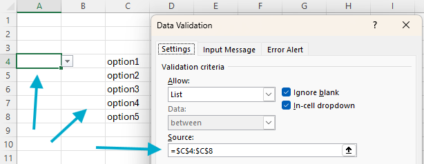
If you skip creating a table, you can enter the list of values in any range inside your workbook before clicking the Data Validation button:
Then, in the Data Validation window, click inside the “Source” field and select the range where you entered the values:
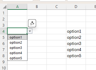
Click ok, and you still get an in-cell dropdown which works quite well:
- You can easily find and modify the list of valid values.
- If you have multiple cells pointing to the same data validation range, they all pick up changes at once.
- You can insert rows within the range and Excel automatically expands the data validation list to include inserted cells:
Even though using a range for the source works well enough, it has a few problems:
- Excel displays the range using coordinates (like $C$4:$C:$8 above). It can become confusing when using multiple ranges as data validation lists.
- If you add items at the bottom of the list, the data validation list does not extend to include them. This can be inconvenient and cause errors.
Skip the named range, but still use a table
A slight variation to the above, is to create a Table, as explained earlier, but skip creating the named range and just click on the cells inside the table to use them as the Source, using cell coordinates.
The downside of this is that the range will not expand when the table expands, when you add to the bottom of your list. In this case, Power Dropdown can help again, because it will always use the full length of your table, even if a range skips some cells.
The “quick and dirty”, and least recommended way
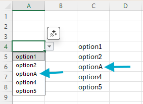
The most obvious (and least recommended) way is to enter a list of values directly in the Source field, like shown below, and hit the OK button (depending on your regional settings, you may replace the semicolons “;” with commas “,”):
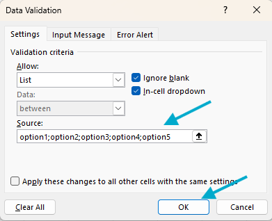
I recommend against using this approach because:
- The list of valid values is hidden within the data validation settings. The only way to see the list or change it is using the same sequence described above and that’s not convenient at all.
- It is possible to apply the same data validation list to multiple cells, but then if you need to change the list you have to apply it everywhere again. Not convenient. And error prone.
More about the Power Dropdown Excel add-in
Power Dropdown doesn’t send any of your data to the cloud, it’s all kept within your file. It only makes in-cell dropdown lists even more powerful; and easier to use.
When you install Power Dropdown, a 3-month trial period starts, during which you can use all features (including Premium). Once the trial is over, you will need a subscription to keep using it. You can also install Power Dropdown from Microsoft Appsource using the links provided below.


If you’d like to learn more about Power Dropdown, click here for the user guide.
You can also download a demo file to experiment with Power Dropdown using a some pre-defined in-cell dropdowns and label/filter rules.